
To analyze Amazon product data with pandas, fetch the recorded history with /api/amazon-product-statistics, turn each price and rank series into a pandas Series, and join them into one DataFrame with a row per day. The series only record changes, so a price holds until the next entry: forward-fill after putting them on a daily index. One credit returns the whole history; the code below builds the frame, then computes 30-day lows, weekly summaries and a chart.
Key Takeaways
- Price series are ["YYYY-MM-DD", minor units] pairs; divide by 100, or by 1 for JPY, to get currency units.
- Several changes can share one day: group by day and keep the last value before building the daily index.
- The series record changes only, so asfreq("D") followed by ffill() gives the price in force on each day.
- salesRankHistory can contain -1 for 'no rank': drop it and forward-fill only short gaps.
- Force numeric dtypes when building frames: an empty series otherwise becomes object dtype and triggers pandas warnings.
Which series go into the DataFrame?
The statistics response carries several histories under data.stats. The three price series share one format and are in minor units; the Buy Box and lowest FBM prices include shipping, the lowest FBA price does not. No-offer periods are removed from the price series, so a forward-filled price can span a stretch where nobody was selling; for the Buy Box, data.buyBoxSellerIdHistory marks those stretches with "-1", the FBA and FBM series have no such marker. The price history guide explains each series.
| Series | Format | Cleaning | Daily fill |
|---|---|---|---|
buyBoxPriceHistory | [day, minor units] | Landed; last per day | ffill |
lowestFBAPriceHistory | [day, minor units] | Item; last per day | ffill |
lowestFBMPriceHistory | [day, minor units] | Landed; last per day | ffill |
salesRankHistory | [time, rank] | Drop -1, last per day | ffill 2 days |
Install pandas and matplotlib next to requests
python3 -m venv .venv
.venv/bin/pip install pandas matplotlib requests
export SELLERMAGNET_API_KEY="your-key-here"
How do I load Amazon price history into pandas?
price_series groups by day before indexing, because two changes on one day would otherwise create a duplicate index; rank_series drops the -1 markers and keeps the last rank per day. daily_frame joins everything and puts it on a daily index. Take the last value per day and forward-fill rather than averaging or interpolating: an interpolated price is one nobody ever paid. get() and new_session() are the helpers from the Python quickstart.
amazon_frame.py - statistics history as a daily DataFrame
"""Statistics history as a daily pandas DataFrame."""
import pandas as pd

from sellermagnet import get, new_session

PRICES = {"buybox": "buyBoxPriceHistory", "fba": "lowestFBAPriceHistory", "fbm": "lowestFBMPriceHistory"}


def price_series(points, scale: int = 100) -> pd.Series:
    """[["YYYY-MM-DD", minor units], ...] -> one value per day in currency units (scale 1 for JPY)."""
    df = pd.DataFrame(points or [], columns=["day", "price"]).astype({"price": "float64"})
    s = df.groupby("day")["price"].last()          # several changes on one day: the last one wins
    s.index = pd.to_datetime(s.index)
    return s / scale


def rank_series(points) -> pd.Series:
    """[["YYYY-MM-DD HH:MM:SS", rank], ...] -> last rank per day; -1 (no rank) dropped."""
    df = pd.DataFrame(points or [], columns=["time", "rank"]).astype({"rank": "float64"})
    df = df[df["rank"] >= 1]
    s = df.set_index(pd.to_datetime(df["time"]))["rank"]
    return s.resample("D").last()


def daily_frame(asin: str, marketplace_id: str, scale: int = 100) -> pd.DataFrame:
    stats = get(new_session(), "amazon-product-statistics", asin=asin, marketplaceId=marketplace_id)["stats"]
    prices = pd.concat({name: price_series(stats.get(key), scale) for name, key in PRICES.items()}, axis=1, sort=True)
    frame = prices.join(rank_series(stats.get("salesRankHistory")).rename("rank"), how="outer").sort_index()
    frame = frame.asfreq("D")
    frame.index.name = "day"
    frame[list(PRICES)] = frame[list(PRICES)].ffill()   # a price holds until the next change
    frame["rank"] = frame["rank"].ffill(limit=2)        # short gaps only: ranks move daily
    return frame


if __name__ == "__main__":
    df = daily_frame("B0CL61F39H", "ATVPDKIKX0DER")
    print(df.tail())
print(df.tail()) - example output
            buybox    fba  fbm  rank
day
2026-09-20  414.99  420.0  NaN  35.0
2026-09-21  414.99  420.0  NaN  57.0
2026-09-22  399.99  420.0  NaN  48.0
2026-09-23  399.99  420.0  NaN  48.0
2026-09-24  399.99  420.0  NaN  35.0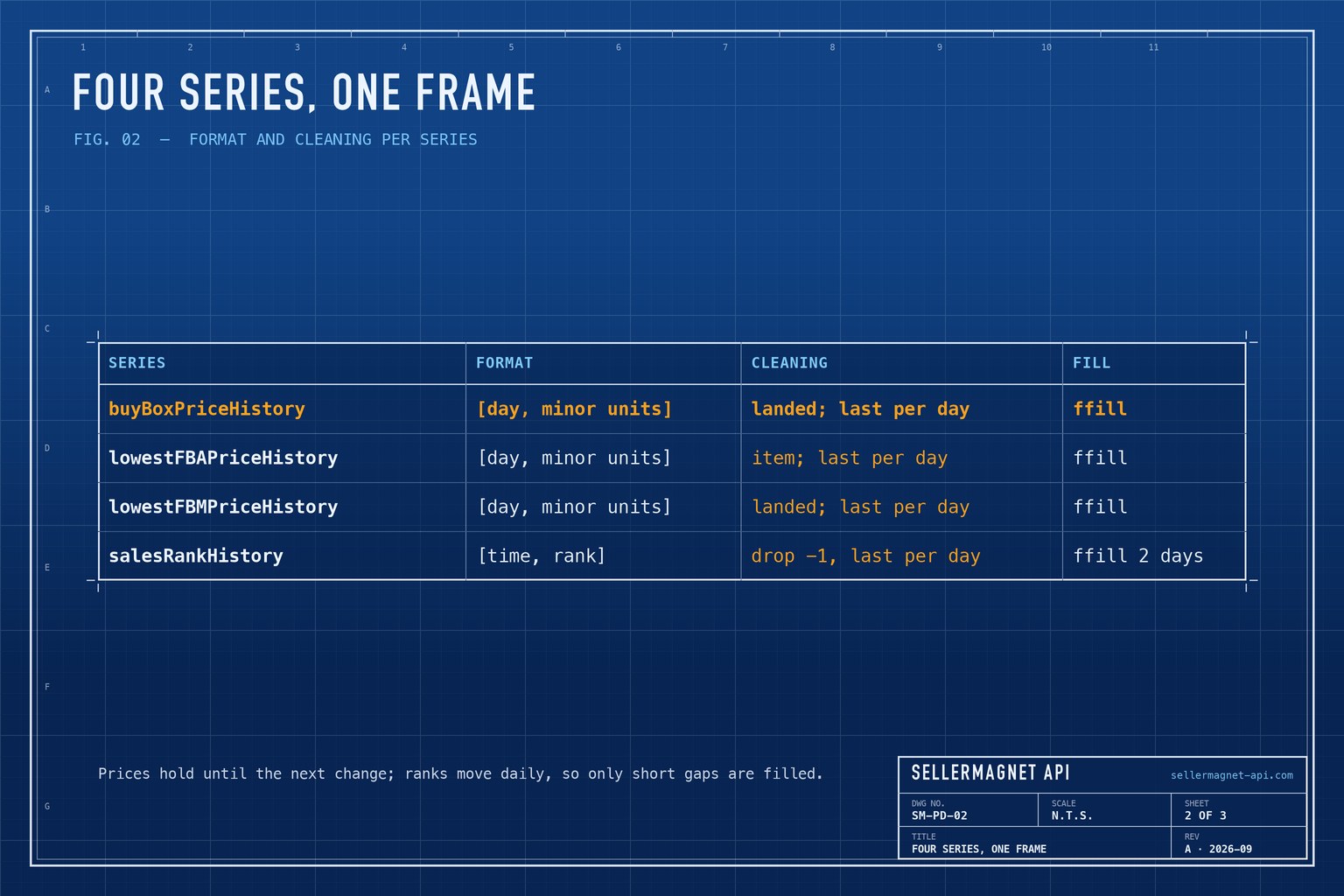
How do I compute 30-day lows and weekly summaries?
With a regular daily index, time-based windows are one-liners. Compute rolling values on the full history and slice afterwards, so the first weeks of your window are not based on partial data. The chart puts price and rank on two axes, with the rank axis inverted so that rank 1 is at the top. resample("W") labels each week by its closing Sunday, so the last row can be a partial week dated a few days ahead.
analyse.py - 30-day low, weekly table, correlation and chart
import matplotlib

matplotlib.use("Agg")                                   # render to a file, no display needed
import matplotlib.pyplot as plt
import numpy as np

from amazon_frame import daily_frame

df = daily_frame("B0CL61F39H", "ATVPDKIKX0DER")
df["low_30d"] = df["buybox"].rolling("30D").min()     # on the full history, then slice
recent = df[df.index >= df.index.max() - np.timedelta64(90, "D")]

weekly = recent.resample("W").agg({"buybox": "mean", "fba": "min", "fbm": "min", "rank": "median"}).round(2)
print(weekly.tail(6))

both = recent[["buybox", "rank"]].dropna()
if len(both) >= 3 and both["buybox"].nunique() > 1:
    print("price vs log(rank) correlation:", round(both["buybox"].corr(np.log(both["rank"])), 2))

fig, ax = plt.subplots(figsize=(10, 4))
ax.plot(recent.index, recent["buybox"], label="Buy Box price")
ax.plot(recent.index, recent["low_30d"], linestyle="--", label="30-day low")
ax.set_ylabel("price")
rank_ax = ax.twinx()
rank_ax.plot(recent.index, recent["rank"], color="grey", alpha=0.5, label="sales rank")
rank_ax.invert_yaxis()                                  # rank 1 at the top
rank_ax.set_ylabel("sales rank")
handles, labels = ax.get_legend_handles_labels()
rank_handles, rank_labels = rank_ax.get_legend_handles_labels()
ax.legend(handles + rank_handles, labels + rank_labels, loc="upper left")
fig.tight_layout()
fig.savefig("B0CL61F39H.png", dpi=150)
weekly.to_csv("B0CL61F39H_weekly.csv")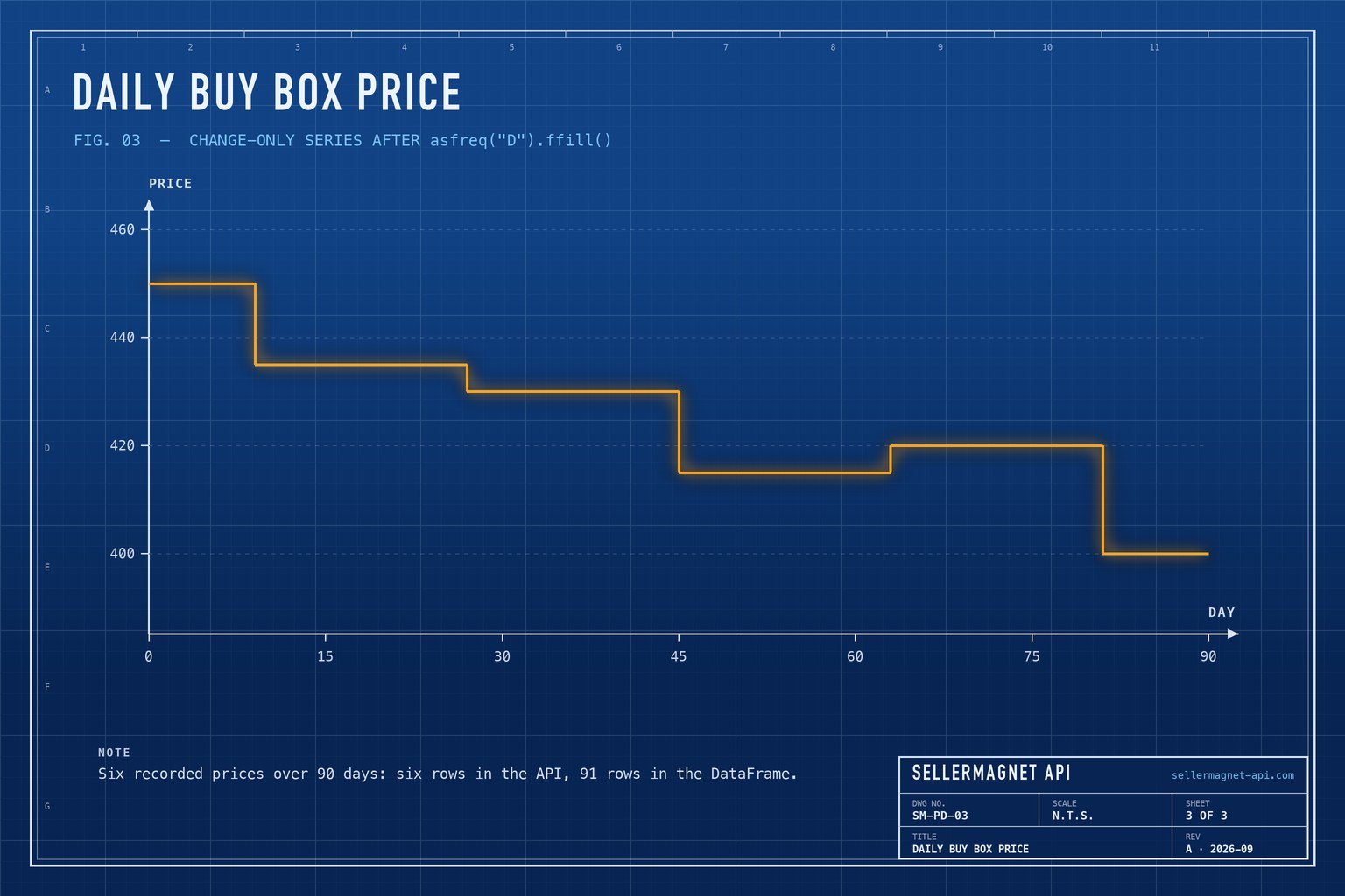
Read the correlation carefully
A positive correlation between price and log rank means lower prices coincided with better (smaller) ranks in this window. Forward-filled days repeat one price, so 91 rows may hold only a dozen distinct prices. It is not proof that the price caused the rank: promotions, stock-outs and seasonality move both. Use it to pick products for a closer look, not as a pricing rule.
Can I analyse many products at once?
Yes: build one frame per ASIN and concatenate a dict of them, which adds the ASIN as an index level: pd.concat({asin: daily_frame(asin, marketplace_id) for asin in asins}, names=["asin", "day"]). Each product costs one credit per refresh. The same response also carries monthly sold units and the rating history, and sales estimates add a units figure. For storing the history instead of recomputing it, see the database guide; for the sales rank itself, the sales rank history guide.
Frequently Asked Questions
Why forward-fill the price history?
The API records a price only when it changes. Forward-filling a daily index gives the price that was in force on each day.
Why is my DataFrame index not unique?
Several price changes can share one day. Group by day and keep the last value before setting the index, as price_series does.
How do I convert the prices to euros or dollars?
Statistics prices are integer minor units: divide by 100, or by 1 for JPY on amazon.co.jp.
What does -1 mean in salesRankHistory?
No rank was recorded at that time. Drop it before resampling, otherwise it distorts medians and charts.
Which marketplaces have this history?
The 11 marketplaces with recorded history, such as amazon.com, .co.uk, .de, .fr and .co.jp. Other marketplaces return a free 400.
Bottom line: one statistics call, a day-level group, a daily index and forward-fill turn change-only history into a DataFrame that pandas can window, resample and plot. The product statistics page has the parameters, and a free account includes 150 credits.


